QGIS

About

QGIS is the central piece of the Boundless Desktop package installation. The well known leading Open Source GIS for desktop, QGIS, is a cross-platform desktop application for viewing, editing, and analysing geospatial data from a variety of (proprietary and open) vector, raster, and database formats.

QGIS’s development is steered by the QGIS Project, which works with hundreds of volunteers and companies (including Boundless) from all over the world, that helps enhance and maintain QGIS.

For convenience, outside the supported scope of Boundless Desktop, the following processing providers are available for QGIS’s Processing framework:

• SAGA 2.3 by http://www.saga-gis.org
• GRASS 7.2 by http://grass.osgeo.org
• Orfeo Toolbox 5.0 by https://www.orfeo-toolbox.org

Quick start guide

This section aims to give you a brief overview about QGIS. We will mainly focus on QGIS’s graphical user interface (GUI) and some of the most common operations like loading data, managing layers and printing a map. For more detailed information on QGIS usage see the tutorials on our learning centre and/or consult QGIS’s official documentation.

For this Quick start, we will be using the Natural Earth data. Please, download Natural Earth Quickstart Kit and unzip it to any folder that you find convenient to access.

QGIS user interface

1. Use any of the available QGIS’s shortcuts on your computer to open QGIS.

   By default, the QGIS GUI should resemble the one presented in the next figure.

   

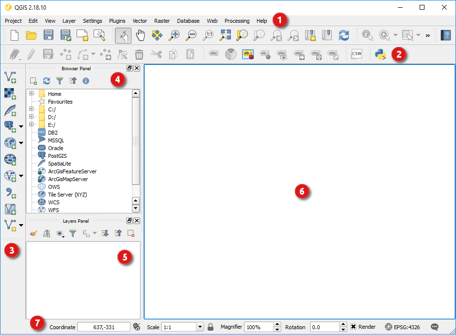
   QGIS Graphical User Interface (GUI)

   As a very basic overview of the default GUI we have:

   • On the top of the screen you will find the menu bar (1). The menu bar provides access to various QGIS features using a standard hierarchical menu.
   • Below it, you will find the main toolbar area (2). Toolbars allow access to most of the same functions as the menus, plus additional tools for interacting with the map. Hold your mouse over the item for a short description of the tool’s purpose. Toolbars can be moved by dragging and dropping them elsewhere and even hidden using View ‣ Toolbars.
   • Another toolbar can be found at the left side of the screen (3). By default, the Manage Layers Toolbar is placed there. This toolbar can be used to load and create data, as we will see later.
   • Next to it, there are two Panels by default: The Browser Panel (4), which is used to browse and load data, and the Layers Panel (5) which is used to toggle layers visibility, setting their relative order, accessing the layer’s properties and much more. Panels can also be moved by drag and drop, or even hidden using View –> Panels.
   • To the right and middle of the screen, you find the map canvas (6) where all visible layers’ geometries will be displayed.
   • At the bottom of the screen you will find the status bar (7) with several useful information and controls for the current map scale, the mouse pointer coordinates, the current Coordinate Reference System’s EPSG code in use, and more.

Loading data

In QGIS, to load data, you can either use the Browser Panel, the Manage Layers Panel or even use your operating system file explorer.

1. Using the Browser Panel, browse to the sample data location, more precisely into the Natural_Earth_quick_start\10m_physical folder. Double-click the folder’s names or click the plus signs next to it to view its contents. Find the ne_10m_coastline.shp shapefile and drag and drop it from the browser to the map canvas. It will load the vector layer.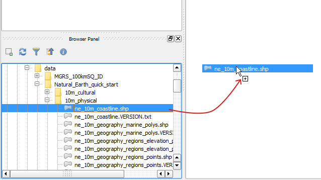

   

   Loading a layer using the Browser Panel

   The layer should now be visible on the map canvas, using a random style. It should also be visible in the Layers Panel list.

   

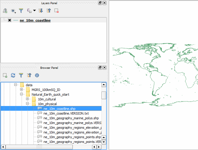
   Successfully loaded layer

2. Let’s open another file, this time using the Manage Layers toolbar buttons. Notice that there is one button for each type of dataset, so we should select the most suitable one. Click on the Add Raster Layer. Then, navigate ito the folder Natural_Earth_quick_start\50m_raster\NE1_50M_SR_W, select the NE1_50M_SR_W.tif file and click Open.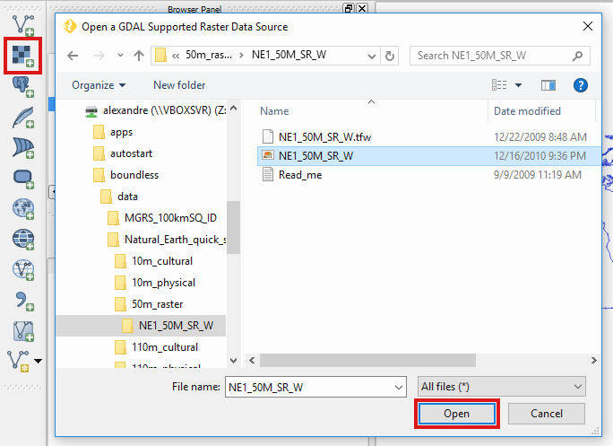

   

   Loading a layer using Add Raster Layer

3. Finally, let’s open an ESRI fileGeodatabase, just because it has a small catch. In the guilabel:Manage Layers toolbar click the Add Vector Layer. In the next dialog, under Source type check the Directory option. Then, making sure that Type is set to ESRI FileGDB, use the Browse button to navigate and select the Natural_Earth_quick_start\10m_cultural \ne_10m_admin_1_states_provinces_geodb.gdb folder. Click choose. Finally, back in the dialog window, click Open to load the layer.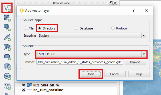

   

   Loading an ESRI FileGeodataBase layer using Add Vector Layer

4. Feel free to add any other data, but bare in mind that you can load several files at once by holding the Ctrl key during file selection in any of the two described methods. Also, you can drag and drop files from your operating system’s file manager (Windows Explorer in Windows or Finder in Mac OS X) into QGIS Map canvas to load them.

Navigating in the map canvas

To navigate the map canvas you can primarily use your mouse wheel. For more precise control over the map canvas, you can also use the Map Navigation Toolbar tools.

1. Position your mouse pointer in an area you that you want to have a closer look, and spin your mouse wheel up to Zoom In. Spin the mouse wheel in the opposite direction to Zoom Out.

2. To pan, just press the mouse wheel down and hold it, move the pointer around and release the wheel once satisfied.

3. As stated above, the Map Navigation Toolbar provides more precise ways to navigate the map.

   Press the Zoom Full button to show the full extent of your data. Now select the Zoom In tool and draw a rectangle around an area of interest using by clicking and dragging the left-mouse-button on the map canvas.

   

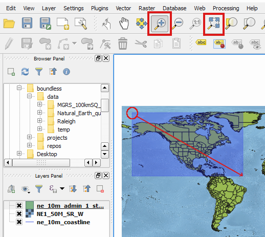
   Loading an ESRI FileGeodataBase layer using Add Vector Layer

4. Notice you can use the Zoom last and Zoom last to undo and redo changes to the map canvas extent

Managing Layers

We have been using the Layers Panel already, but let’s have a deeper look into it’s potential.

1. Select a layer by clicking on its name on the layers list/legend. The layer will become the active layer, meaning that many layer specific tools and actions will apply to that layer in particular. For example, select the ne_10_coastline layer and, in the Map Navigation Toolbar, click the Zoom to Layer button. This will zoom the map canvas to the full extent of a particular layer.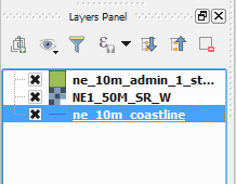

   

   Layer active in the Layers Panel

2. You can change the order of the layers (and consequently their rendering order) by dragging them up and down in the Layers. Do this making sure to put the raster layer at the bottom, the polygons layer above it, and the line layer at the top.

   

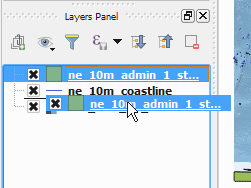
   Changing the order of the layers

3. You can change the visibility status of the layers by (un)checking the small checkbox next to its name. Give it a try and see the result in the map canvas. (Make sure to keep all layers visible in the end)

   

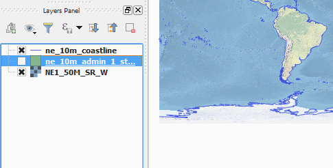
   Changing the layers’ visibility

4. By double-clicking the layer name in the Layers Panel, or right-clicking and selecting properties, you will open the layer’s properties. Double-click the ne_10m_admin_1_states_provinces layer, navigate to the Style tab. There you can change how the layer will be displayed in the map. Click the Simple fill in the symbols layers list, and in the Fill Fill type select No brush. Press Ok to apply the changes and close the properties dialog.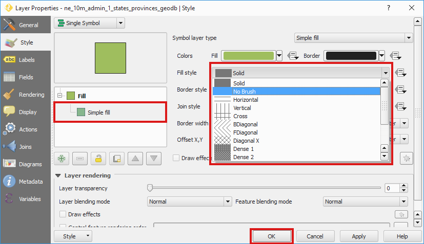

   

   Changing the layers’ style in the properties dialog

   At this time you might want to save your project.

5. Go to Project ‣ Save or hit Ctrl+S. Choose the destination folder where your project will be saved, type in a sugestive name and click Save.

Exploring data’s attributes

To make proper use of the dataset, one should know its attributes. Let’s see how to retrieve the attributes of our layers.

1. Make sure the ne_10m_admin_1_states_provinces layer is still active and in the Attributes toolbar (if not visible, go to View ‣ Toolbars), select the Identify tool. Then, click the map over one of the geometries of the layer. The Identify Results Panel will show up, where you can see the feature’s fields and respective values. (You may need to expand the panel a bit to see it all).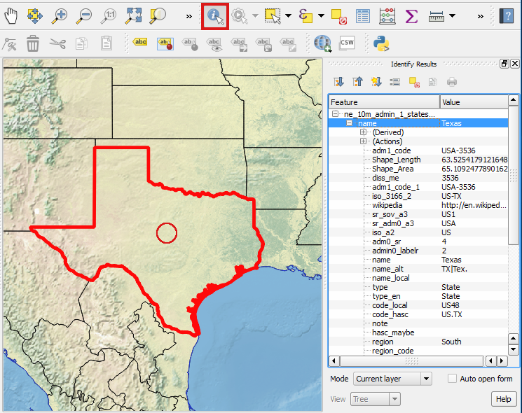

   

   Seeing layer’s attributes using the identify tool in a feature

2. You can also see all attributes of your layer in its attributes table. Having the ne_10m_admin_1_states_provinces layer selected, click the Open Attributes table in the Attributes toolbar (or right-click the layer’s name in the Layers Panel and choose Open Attribute Table ). The layer’s attribute table will show up.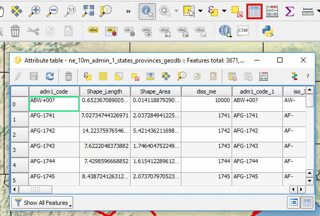

   

   Seeing layer’s full attributes using the attribute table

3. In the attribute table, use the mouse wheel to quickly scroll up and down the attributes, or the scroll bar to move horizontally.

4. Select one feature by clicking its id number at the left side of the feature’s row of attributes. Then, use the Zoom to Selected Rows tool at the top of the attribute table to zoom the map to that particular layer.

   

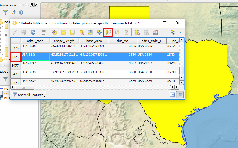
   Selecting a row in the attribute table and zooming to it’s feature

5. Repeat step 4 selecting several rows by holding the Ctrl key while clicking the id numbers. In the end, make sure to deselect all features using the Deselect All button in the attribute table.

Add simple labels

Now that we already know our data attributes, let’s use one as a label for our geometries.

1. Go back to the ne_10m_admin_1_states_provinces properties menu by double-clicking its name in the Layers panel. Go to the Labels tab, and select Show labels for this layer. Then, in the Label with combobox select the abbrev field. Press Ok to apply the changes, close the properties dialog and see how it looks.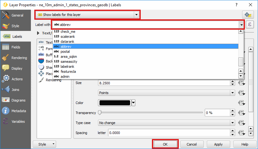

   

   Layer’s properties Label tab

Print a simple map

Now let’s see how to print a very simple map with the layers that we have loaded. In QGIS, you can have as many map layouts (a.k.a. print compositions) as you like, and you can manage them in the Print Composer Manager.

1. Once you are satisfied with the map’s looks, click the New Print Composer button in the File toolbar, type a representative name for the composer and click Ok.

   

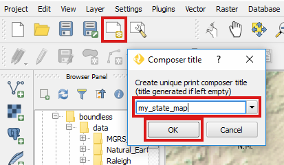
   Creating a new composer and choosing a name

2. The print composer will open with an empty page. To add a map item, click the Add Map in the Toolbox toolbar and draw a rectangle covering most of the page by clicking and dragging over it. The map content should appear.

   

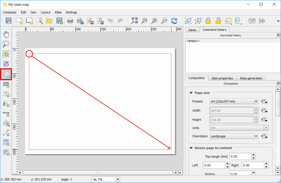
   Adding a map item to the print composer page

3. You can adjust the map item position and size by clicking and dragging the corner and side handles.

4. You can also adjust the map extent using the Move item content tool. While this tool is selected, you can pan the map content clicking and dragging inside of it, and change its scale using the mouse wheel. More precise controls to set the map item position, size, scale and extent can be found in the Item properties tab/panel.

   

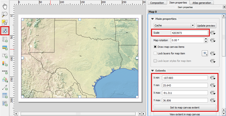
   Adjusting map item’s scale and extent

5. Now that we are satisfied with our very minimalist map, let’s export it. In the Composer toolbar, click Export to PDF. Choose a location and name for your PDF file and click Ok.

Obviously, we could do more complex maps by adding other items like legends, labels and images. Please see our learning centre to learn how to work with them. Also, if you have interessed, have a look into this QGIS Map Gallery.

QGIS Browser

Alongside with QGIS you will find QGIS Browser, another QGIS standalone application in the Boundless Desktop folder. QGIS Browser can be used to browse the datasets quickly on your local computer, network or remote services. You can see its metadata, preview its geometries and see the attribute table.

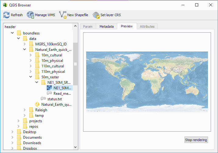
Standalone QGIS browser GUI

Online resources

• Official Site: http://www.qgis.org
• Documentation: http://docs.qgis.org/2.18/en/docs/index.html
• Official Plugins Repository: http://plugins.qgis.org/plugins/